Lab 7

Lab Tasks

1. Estimate Drag and Momentum

I estimated the drag and momentume values necessary for the A and B matricies using a step response. I accomplished this by driving my robot towards a wall at a constant motor input while the ToF sensor collected distance measurements. From this data, I calculated the velocity and plotted it to find the 90% rise time. I selected my step input u(t) based on my calibration factor such that one wheel was operating at 250 PWM. This input was approximately 72% of the maximum PWM. This PWM value allowed for my robot to move as fast as possible while still moving in a straight line for long distances.

To conduct there trials I implemented the following two cases into my code to initiate the trial and collect data.

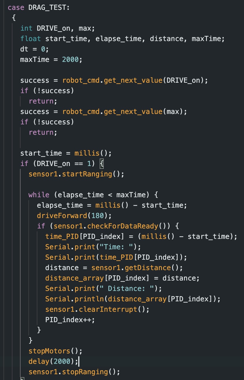
DRAG_TEST

This case clears all previous data, starts my front ToF sensor, initiates storage of time data, and sets DRIVE_on to 1 (this is initialized as 0 to keep the car off until the command is called). For the DRAG_TEST case, the command inputs consist of the DRIVE_on value and the array size “max” for data collection.

GET_DRAG_TEST_DATA

This case transmits the collected data to my computer via Bluetooth. While designing the GET_DRAG_TEST_DATA case, I decided that the relevant information that I needed to send to Jupyter Notebook consisted of: time, distance (mm), and PWM value. This case was formatted the same way as in Labs 5+6 for sending data.

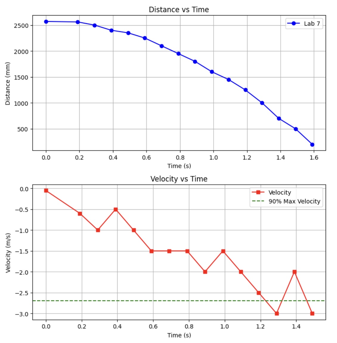
Collecting data over a period of two seconds, I collected the following data:

In order to calculate the drag and momentum, I used the following equations below:

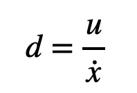
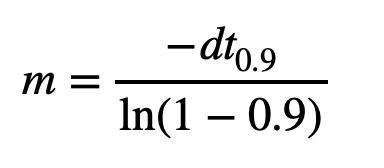
From my trials using a PWM value of 180, I found that my 90% value for speed is 2.74968 m/s which occurs at approximately 1.237 seconds. Using the aforementioned equations, I got the following values for drag and momentum.

\(d = 1 / 2.74968 = 0.36368\) \(k = (-0.36368 * 1.237)/ln(0.1) = 0.19537\)

2. Initialize Kalman Filter (Python)

I found my A and B matricies using the following formula and my calculated values for d (drag) and m (momentum):

\[A = \begin{bmatrix} 0 & 1 \\ 0 & -d/m \end{bmatrix}\] \[B = \begin{bmatrix} 0 \\ 1/m \end{bmatrix}\]

These matricies were calculated as seen below (after converting to the appropriate units)

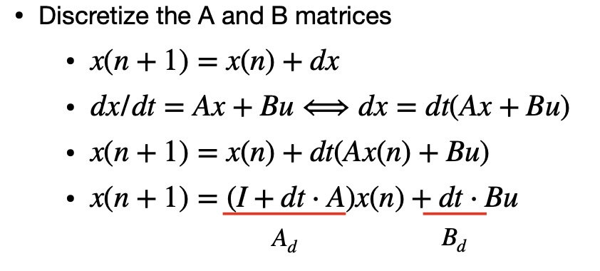
\[A = \begin{bmatrix} 0 & 1 \\ 0 & -1.8615 \end{bmatrix}\] \[B = \begin{bmatrix} 0 \\ 5118.4931 \end{bmatrix}\]

Once I had my A and B matrcies, I had to discretize them. I used the following methodolgy which was presented in class to accomplish this task.

While initially, I planned to find the sampling time for the two matricies Ad and Bd, by finding the difference between timestamps, I found that this data was unreliable. As such I ended up using an average of values colleted across a loop. This in turn left me with an average sampling time of roughly 0.0872 seconds.

Below, is the calculations I completed to find the discretized Ad and Bd matricies.

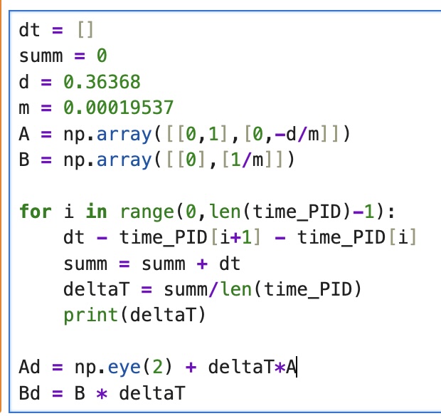
\[Ad = (I + dt * A)\] \[Ad = \begin{bmatrix} 1 & 0 \\ 0 & 1 \end{bmatrix} +(0.0872)* \begin{bmatrix} 1 & 0 \\ 0 & -1.8615 \end{bmatrix}\] \[Ad = \begin{bmatrix} 1 & 0.0872 \\ 0 & 0.8376 \end{bmatrix}\] \[Bd = (dt * B)\] \[B = (0.0872) * \begin{bmatrix} 0 \\ 5118.4931 \end{bmatrix}\] \[B = \begin{bmatrix} 0 \\ 446.33 \end{bmatrix}\]

I used the following code in python to find the value for dt.

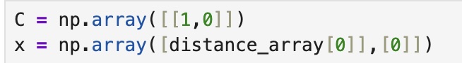
In order to find the C matrix, I used the following code in python

Lastly, I had to find the process noise and sensor noice covariance matricies. I refernced the slides from Lecture 14 to identify these equations.

\(\sigma_1 = \sqrt{(10mm)^2 * (1/0.0872)} = 33.864 mm\) \(\sigma_2 = \sqrt{(10mm/s)^2 * (1/0.0872)} = 33.864 mm\) \(\sigma_3 = 20 mm\) \(\sum_{i=1}^{u} = \begin{bmatrix} (33.864)^2 & 0 \\ 0 & (33.864)^2 \end{bmatrix}\)

\[\sum_{i=1}^{z} = \sigma_3^2 = ((20mm)^2)\]

3. Implement and Test Kalman Filter in Jupyter (Python)

I implemented the following function into my python code to perform the Kalman Filter.

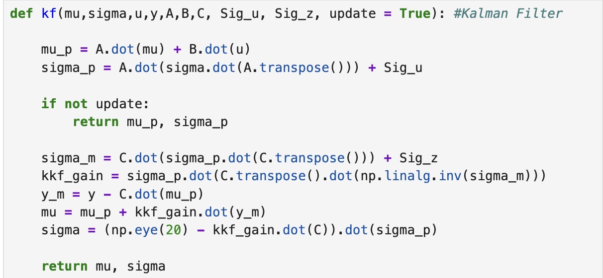
This code predicts and returns values for mu and sigma. If theres not a new ToF sensor reading, the Kalman Filter will return the predicted values.

References

For this lab I primarily referenced Stephen Wagner, Daria Kot, and Mikayla Lahr’s labs from the past year. I also used ChatGPT for help with syntax to properly format matricies and equations in my webpage.